Although all of Mendel’s pea plant characteristics behaved according to the law of independent assortment, we now know that some allele combinations are not inherited independently of each other. Genes that are located on separate, non-homologous chromosomes will always sort independently. However, each chromosome contains hundreds or thousands of genes, organized linearly on chromosomes like beads on a string. The segregation of alleles into gametes can be influenced by linkage, in which genes that are located physically close to each other on the same chromosome are more likely to be inherited as a pair. However, because of the process of recombination, or “crossover,” it is possible for two genes on the same chromosome to behave independently, or as if they are not linked. To understand this, let us consider the biological basis of gene linkage and recombination.

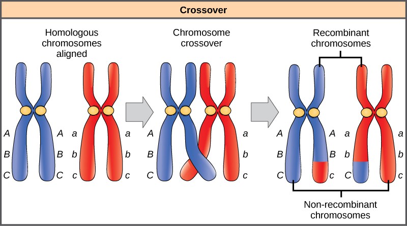
Homologous chromosomes possess the same genes in the same order, though the specific alleles of the gene can be different on each of the two chromosomes. Recall that during interphase and prophase I of meiosis, homologous chromosomes first replicate and then synapse, with like genes on the homologs aligning with each other. At this stage, segments of homologous chromosomes exchange linear segments of genetic material (Figure 1). This process is called recombination, or crossover, and it is a common genetic process. Because the genes are aligned during recombination, the gene order is not altered. Instead, the result of recombination is that maternal and paternal alleles are combined onto the same chromosome. Across a given chromosome, several recombination events may occur, causing extensive shuffling of alleles.

When two genes are located on the same chromosome, they are considered linked, and their alleles tend to be transmitted through meiosis together. To exemplify this, imagine a dihybrid cross involving flower color and plant height in which the genes are next to each other on the chromosome. If one homologous chromosome has alleles for tall plants and red flowers, and the other chromosome has genes for short plants and yellow flowers, then when the gametes are formed, the tall and red alleles will tend to go together into a gamete and the short and yellow alleles will go into other gametes. These are called the parental genotypes because they have been inherited intact from the parents of the individual producing gametes. But unlike if the genes were on different chromosomes, there will be no gametes with tall and yellow alleles and no gametes with short and red alleles. If you create a Punnett square with these gametes, you will see that the classical Mendelian prediction of a 9:3:3:1 outcome of a dihybrid cross would not apply. As the distance between two genes increases, the probability of one or more crossovers between them increases and the genes behave more like they are on separate chromosomes. Geneticists have used the proportion of recombinant gametes (the ones not like the parents) as a measure of how far apart genes are on a chromosome. Using this information, they have constructed linkage maps of genes on chromosomes for well-studied organisms, including humans.

Mendel’s seminal publication makes no mention of linkage, and many researchers have questioned whether he encountered linkage but chose not to publish those crosses out of concern that they would invalidate his independent assortment postulate. The garden pea has seven chromosomes, and some have suggested that his choice of seven characteristics was not a coincidence. However, even if the genes he examined were not located on separate chromosomes, it is possible that he simply did not observe linkage because of the extensive shuffling effects of recombination.

Epistasis

Mendel’s studies in pea plants implied that the sum of an individual’s phenotype was controlled by genes (or as he called them, unit factors), such that every characteristic was distinctly and completely controlled by a single gene. In fact, single observable characteristics are almost always under the influence of multiple genes (each with two or more alleles) acting in unison. For example, at least eight genes contribute to eye color in humans.

In some cases, several genes can contribute to aspects of a common phenotype without their gene products ever directly interacting. In the case of organ development, for instance, genes may be expressed sequentially, with each gene adding to the complexity and specificity of the organ. Genes may function in complementary or synergistic fashions, such that two or more genes expressed simultaneously affect a phenotype. An apparent example of this occurs with human skin color, which appears to involve the action of at least three (and probably more) genes. Cases in which inheritance for a characteristic like skin color or human height depend on the combined effects of numerous genes are called polygenic inheritance.

Genes may also oppose each other, with one gene suppressing the expression of another. In epistasis, the interaction between genes is antagonistic, such that one gene masks or interferes with the expression of another. “Epistasis” is a word composed of Greek roots meaning “standing upon.” The alleles that are being masked or silenced are said to be hypostatic to the epistatic alleles that are doing the masking. Often the biochemical basis of epistasis is a gene pathway in which the expression of one gene is dependent on the function of a gene that precedes or follows it in the pathway.

An example of epistasis is pigmentation in mice. The wild-type coat color, agouti (AA) is dominant to solid-colored fur (aa). However, a separate gene C, when present as the recessive homozygote (cc), negates any expression of pigment from the A gene and results in an albino mouse (Figure 2). Therefore, the genotypes AAcc, Aacc, and aacc all produce the same albino phenotype. A cross between heterozygotes for both genes (AaCc x AaCc) would generate offspring with a phenotypic ratio of 9 agouti:3 black:4 albino (Figure 2). In this case, the C gene is epistatic to the A gene.