
2 Gradients
Having laid the groundwork of understanding where our signal is coming from, we could go in one of two directions. We could start talking about relaxation, which is the process of returning to equilibrium after excitation and releasing the energy that becomes our signal. Or we could start talking about the I part of MRI — imaging. I find it easier to take the latter path. Before continuing with the MR part of the story (relaxation), I like to pause and talk about gradient coils: what they are and how we use them to turn NMR into MRI. My motivation for following this path is that we’re following the path of a pulse sequence: a gradient is often applied during excitation, and gradients are generally applied (“played”) to add some spatial information encoding while we’re waiting for relaxation processes to happen.
When we’re doing this class in person, we pause here to outline the Huettel textbook and talk about how the trajectory of this class does and doesn’t match the trajectory of that textbook, which is the best traditional reference I know for understanding the imaging process. Here are pdfs of parts of Ch. 3 and Ch. 4, so they’re handy for the outlining exercise. But purchasing and referring back to the entire textbook is a great choice for most students of MRI!
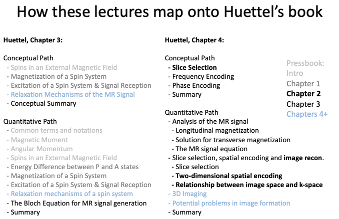
Huettel, 2nd Edition, Chapter 3
Huettel, 2nd edition, Chapter 4
First, the physics of what a gradient is and what it does to the sample:
This section is evolving — these new slides hopefully provide slightly better illustrations than the old ones:
Slice selection, conceptually:
Exercises
Next, how do we use gradients for slice selection?
Exercises
2.1 What does “slice selection” mean?
2.2 Imagine you are applying an RF pulse while a gradient is turned on, with the intention of selecting a slice. If you don’t change the bandwidth of the pulse, but you increase the strength of the gradient, will your slice get thicker or thinner?
These next 2 parts are really 1, but the first time through … the movies didn’t get captured. So it’s broken into 2 parts.
… and the 2nd part, with movies (and homework).
Exercises
3.1. The arithmetic is annoying … but go ahead and fill out the table of slice thickness, location, and orientation shown on the last slide.
3.2. What parameter in the table should be adjusted to do the experiment at a different field strength?
3.3. Which image is acquired during an echo? (Note: the illustration in the video is a bit messed up because in the image at left, color indicates the relative phase at each location, while in the image at right, color indicates the intensity of the signal at each location. In the slides, the illustration is corrected so color always indicates phase and the saturation indicates ‘proton density’ — how much sample is at each location.)
3.4. Which image is closer to the center of k-space?
3.5. What is k-space, anyway?
In https://github.umn.edu/caolman/MRIsimulations.git/demos, there’s code called FLASH_oneLine.py that generates read_out.mp4, illustrating the phases at each location in the sample as gradients with different slopes are left on, and how the vector sum of all of those phases results in an induced signal in the coil that comes to an “echo” when the gradient history is balanced:
Exercises
