
15 Perspectives on the Fourier transform
I get so excited when Fourier transforms come up because there are so many truths that are useful! But it’s another tangled web of facts. So here are some things I love about Fourier transforms (and background facts that you need to work with Fourier transforms).
Quadrature pairs
When something is rotating in 2D, it can be projected onto x- and y-axes. By convention, theta is the angle that describes the direction that something is pointing in, it’s measured relative to the positive x-axis, and it rotates counter-clockwise. The part that’s projected onto the horizontal axis is “cosine-phase” — it starts positive, crosses 0, goes negative, comes back. The part that’s projected onto the vertical axis is “sine phase” — it starts at 0, grows, then crosses back through θ to negative territory.
1D Fourier Transforms
Here is an interactive Colab notebook for exploring 1D Fourier transforms of different time series.
Complex numbers
You can get the gist of Fourier transforms without using complex numbers, but to do the math, you need to be acquainted with complex numbers. Folks who thrived in Complex Analysis would find my descriptions here inadequate, I am sure … but here’s how I think of them.
i is the marker for complex numbers (or j if you’re an engineer). It is defined as the square root of -1. That’s impossible, right? When you square a number, you multiply it by itself … a negative number times a negative number is a positive number … there’s no way to get a negative number when you square something, right? But i2 = -1. At some point I knew how this definition was derived, but I’ve long since forgotten. I’m sure there’s much more, but because I don’t do math for a living, to me i is a marker for something that is spinning or cyclical. Let me explain!
It’s standard to use z to represent a complex number, which is a number with 2 parts:
z = x + iy
x is the real part of the complex number, y is the imaginary part. That’s just a definition, but now we’re going to think of x as a distance on one axis and y as a distance on another axis.
If we look at that quadrature pair movie, we can see how complex numbers might be used to describe things that are spinning. The point at the tip of the black line is z — a complex number. I could tell you how to find the point at the tip of that line two ways: either I could tell you to travel a certain distance along the x-axis and then a certain distance up parallel to the y-axis … or I could tell you to travel in a certain direction for a certain distance (that’s a polar coordinate system).
So complex numbers, as it turns out, can be described two ways. They have a magnitude, written as |z|, and a direction, θ (the angle between z and the x-axis). At any given moment, z has a projection onto the x-axis: x = |z|·cos(θ). That’s called the “real” part. The projection to the y-axis is y = |z|·sin(θ). Now, if we define the y-axis as the “imaginary” axis, then i becomes just a marker for the part that goes on the vertical axis:
z = x + iy = |z|·cos(θ) +i|z|·sin(θ)
Below, there’s a little more detail on how to multiply complex numbers together and how to calculate |z|, and i‘s definition as the square root of -1 becomes more meaningful. For understanding Fourier transforms, however, the most important thing is to think of the real part x as the part of a signal that is “cosine-phased” and y is the part of a signal that is “sine-phased”. If θ increases with time, z will spin.
eiθ = cos(θ) + isin(θ)
Again, there’s a derivation for that definition that someone who loved Complex Analysis could tell you immediately. I think of it as a mathematical convenience or short hand for representing things that are spinning or cyclical. Instead of writing z = |z|·cos(θ) +i|z|·sin(θ), you can take advantage of Euler’s identity and write z = |z|eiθ. Wolfram has a good section about the basics of complex numbers, and how the eiθ = cos(θ) + isin(θ) definition is directly related to this computation of phase.
Connection of the above ideas to the equations we’ll use for MRI
For protons or spin isochromats (collections of protons all at exactly the same frequency), eiθ describes their precession. This precessing net magnetization induces a signal in a coil. That signal is oscillating. When is it bigger and when is it smaller? It depends on your perspective, or what direction the isochromat was pointing at whatever time we defined as 0. The more important question is what is the relative phase of that signal at any given time, which is theta.
1D Fourier transforms
OK, now we’re armed with the background we need to do some Fourier transforms. I always use timeseries when I do 1D Fourier transforms, because it seems like the most obvious example, but the transform is just math and not tied to any particular physical thing.
Real-world examples of things that do Fourier transforms all the time are the basilar membrane in your inner ear, which vibrates in different places when different frequencies oscillate your ear drum, and sound systems that let you increase or decrease the treble or bass on a soundtrack. You take a complicated pattern, break it down into its components … maybe manipulate them … and then put it back together.
At a recent talk by Brad Voytek I saw the best illustration yet, which I’ve stolen and pasted below, until I have a chance to make my own.
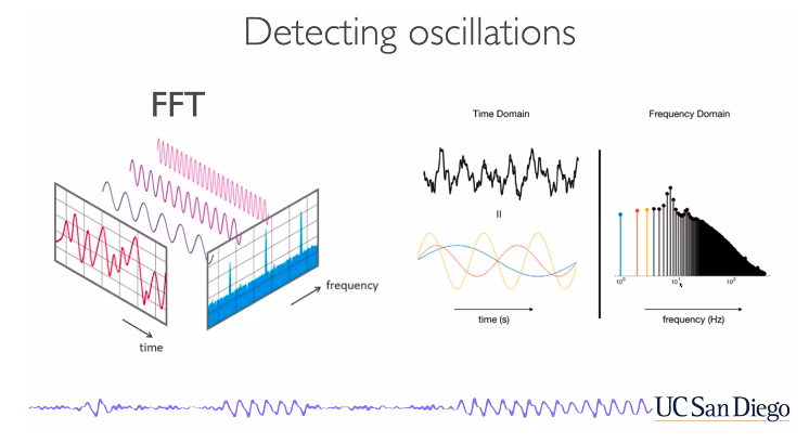
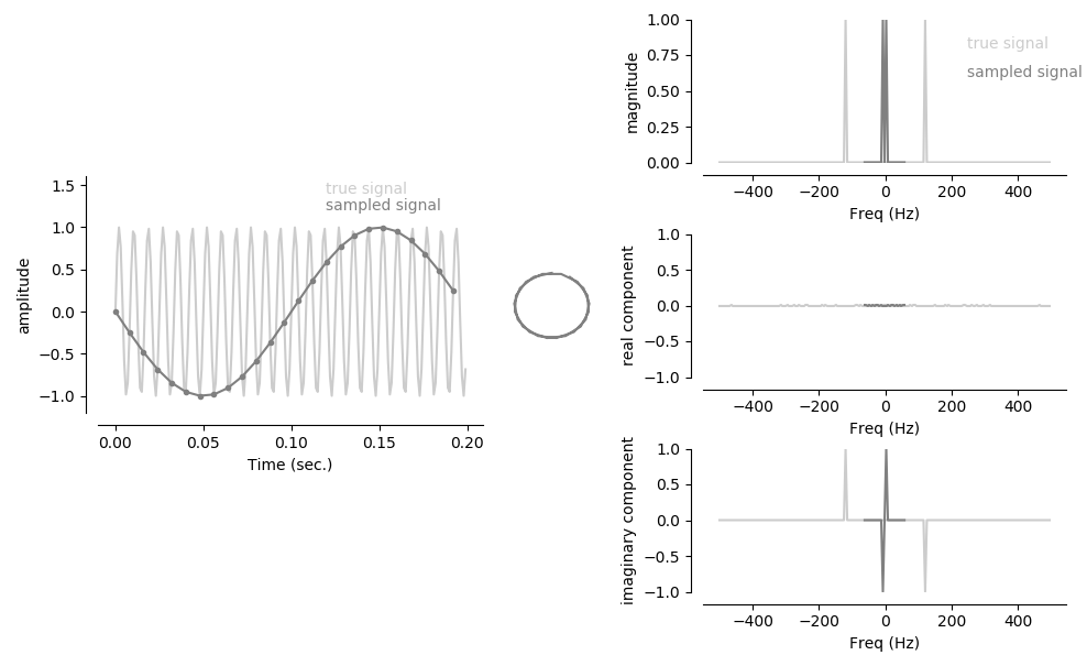
But really, I think the best way to experience Fourier transforms is to play with code, so I’ve written some demo code that lets you play with the signal shape and phase and sampling resolution and see what happens to the Fourier transform. It is hosted as a Colab notebook here, and there’s also a copy in the FFT folder of https://github.umn.edu/caolman/MRIsimulations. It generates images like the one below, to get used to the real and imaginary parts of a Fourier transform and the consequences of sampling rate.
Filtering and convolution — not yet written!
[This will be a basic tutorial on convolution and how convolution in time domain is multiplication in frequency domain.]
2D Fourier transforms
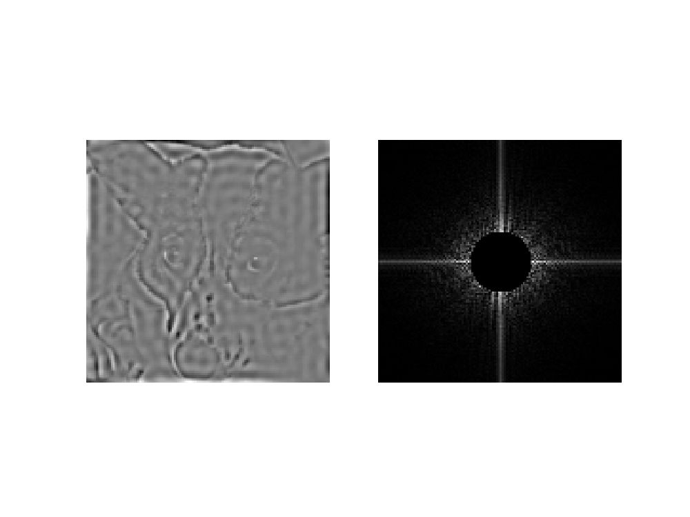
Code for exploring FFTshift and the structure of 2D matrices is https://github.umn.edu/caolman/MRIsimulations/FFT/FFT2_demo.py and generates pictures like the one below. An interactive Colab version of that is here.
Filtering again
Examples of filters in the Fourier domain and the artifacts they create in the image domain. One will be a spike; one will be T2* decay causing blurring; one will be imbalances in every-other line or every-fourth line that creates ghosting.
Hermitian symmetry and complex conjugates
A complex number has real and imaginary parts and is written as a + ib (or a + jb, if you’re an engineer and use j instead of i for √-1). ‘a’ indicates the real part of the number, and ‘b’ indicates the imaginary part of the number.
If z = a + ib is a complex number, then its conjugate, z*, is a – ib. The magnitude of a complex number is defined as √(z)(z*), which works out to √a2+b2. For whatever reason, I get a kick out of working z2 out the hard way: (z)(z*) = (a + ib)(a – ib) = a2 + iab – iab –i2b2 = a2 -(-1)(b2) = a2+b2. So I always think of a complex number as the hypotenuse of a triangle that is a on one side and b on the other.
While we’re picturing triangles … they have angles. So complex numbers also have phases (directions). The phase of the complex number is defined as tan-1(b/a). When b and a are both positive, it’s again easy to picture this an angle inside a right triangle, like above. But, like the math for computing magnitude … the math is right all the time, even though complex numbers in other quadrants aren’t tidy little triangles.
Finally … Hermitian symmetry. If you have a matrix of complex numbers, it has Hermitian symmetry if each point is the complex conjugate of its counterpart on the other side of the matrix. It’s easier to draw than describe:
| a + iz | b + iy | c + ix | d + iw | e + iv |
| f + iu | g + it | h +is | k + ir | l + iq |
| m + ip | n + io | 0 | n – io | m – ip |
| l – iq | k – ir | h – is | g – it | f – iu |
| e – iv | d – iw | c – ix | b – iy | a – iz |
So if you know half the matrix, you can predict the other half … I didn’t run out of alphabet filling out a 5 x 5 matrix, even though each cell has 2 letters and I would have needed 50 letters for a matrix of complex-valued numbers that didn’t have Hermitian symmetry. Note that I had to skip i and j, too, so I put a 0 in the middle …
